NuthKaab Coreg vs Gradient Descent Coreg
DEM coregistration is an important step in improving the quality of a DEM by eliminating horizontal shift and vertical bias. However, it can be time-consuming, particularly for large datasets and global applications such as the SNOWDEPTH project.
In the past few months, I have found that the implementation of NuthKaab coregistration in xDEM is not fast enough for ICESat-2 datasets. As a result, I have developed a new method called ‘Gradient descent Coregistration,’ which works similarly to ICP (Iterative Closest Point) but is significantly faster. I am eager to receive professional input to make this method more robust and useful for others.
The purpose of this section is:
- to compare the performance of NuthKaab coregistration and ‘Gradient descent Coregistration’ on ICESat-2 datasets.
- In addition, I will consider the possibility of extending ‘Gradient descent Coregistration’ to other scenarios beyond ICESat-2 point coregistration.
- Finally, I will explore the footprint problem: should I treat the point measurements of ICESat-2 as a footprint (zonal statistics) or using point interpolation.
import pandas as pd
import geopandas as gpd
import xdem
import xdem_pt
import importlib
import pyproj
from xsnow.godh import load_gdf,best_shift_px,get_dh_by_shift_px_gdf,get_dh_by_shift_px_dem,get_dh_dem,dem_difference_plot, best_footprint,get_dh_by_footprint
from xsnow.misc import df_from_dem
from xsnow.goplot import final_histogram
# Loading the dataset.

# 1 ICESat-2 snow free measurements.
sf_gdf = pd.read_csv('snow_free_land_gdf.csv', sep='\t', encoding='utf-8')

# 2 DTM 10 exmaple (10 m Norway DTM-10)
fid_dtm10 = r'\\hypatia.uio.no\lh-mn-geofag-felles\projects\snowdepth\data\DEM\Norway\DTM10_UTM33\6603_3_10m_z33.tif'
dtm_10_ = xdem.DEM(fid_dtm10).reproject(dst_crs=pyproj.CRS(32633),dst_res=(10,10))
dtm_10 = dtm_10_ + xdem.DEM('no_kv_HREF2018B_NN2000_EUREF89.tif').reproject(dtm_10_,resampling='bilinear')

# 3 DTM 1 exmaple (1 m Norway DTM-1)
fid_dtm1 = r'\\hypatia.uio.no\lh-mn-geofag-felles\projects\snowdepth\data\DEM\Norway\DTM1_11-11_UTM33\33-112-114.tif'
dtm_1_ = xdem.DEM(fid_dtm1).reproject(dst_crs=pyproj.CRS(32633),dst_res=(1,1))
dtm_1 = dtm_1_ + xdem.DEM('no_kv_HREF2018B_NN2000_EUREF89.tif').reproject(dtm_1_,resampling='bilinear')

# subset snow free measurements
from xsnow.godh import load_gdf
sf_subset_dtm10 = load_gdf(sf_gdf,dtm_10,z_name='h_te_best_fit')
sf_subset_dtm1 = load_gdf(sf_gdf,dtm_1,z_name='h_te_best_fit')

print(f'The length of sf_subset_dtm10: {len(sf_subset_dtm10)} points')
print(f'The length of sf_subset_dtm1: {len(sf_subset_dtm1)} points')
The length of sf_subset_dtm10: 20291 points
The length of sf_subset_dtm1: 1113 points
The Main Challenges of Applying NuthKaab Coreg on ICESat-2
NuthKaab estimates the ‘shift matrix’ iteratively by solving a cosine equation that models the direction in which the DEM is most likely offset.
- (1) However, this process requires the calculation of ‘slope’, ‘aspect’, and ‘curvature’, which can be time-consuming and resource-intensive, especially if the DEM has a fine resolution. In fact, the computational cost of NuthKaab coregistration grows exponentially as the resolution of the DEM increases.
- (2) In addition, NuthKaab is a statistical method that requires a large sample of points (e.g. at least 1000-2000) to work accurately. If there are too few points available in the ICESat-2 dataset (which is often the case with fine DEMs), NuthKaab may not work properly or may produce incorrect results.
Below, I have provided three examples to illustrate these challenges.
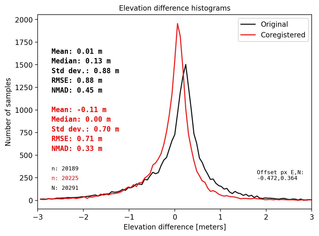
- (a) NuthKaab coregistration works well on a normal DEM with sufficient points.
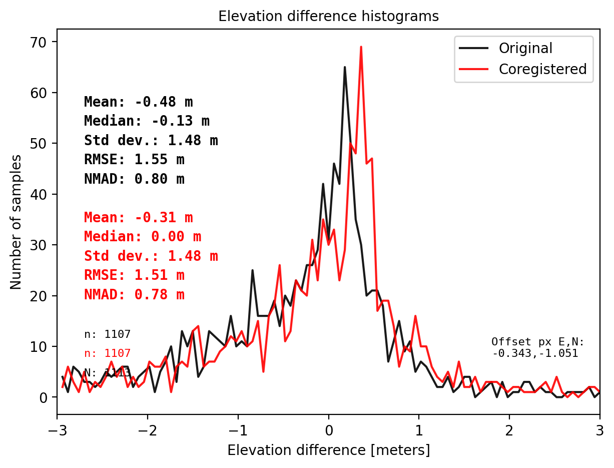
- (b) NuthKaab takes longer and produces incorrect results on a fine DEM with fewer points.
- (c) NuthKaab fails completely when there are not enough points (e.g. less than 500).
NuthKaab Coreg
%%time

# (a) NuthKaab Coreg examples of DTM10. It works well on normal DEMs.
results_nk_10 = get_dh_dem(dtm_10,sf_subset_dtm10,range=(-3,3),perc_t=99.75,std_t=None,mask_highcurv=False,verbose=False)
Warning: There is no curvature in dataframe. Set mask_highcurv = True for more robust results and costs more time
CPU times: total: 35.3 s
Wall time: 35.3 s
%%time

# NuthKaab example on DTM1, it consumes more time on DTM1, and bad coreg due to sample size.
result_nk_1 = get_dh_dem(dtm_1, sf_subset_dtm1,range=(-3,3),perc_t=99.75,order=1,mask_highcurv=False,verbose=False)

# The STD, RMSE, NMAD do not improve after NuthKaab Coreg.
# Even the bias is not relieable becasue the samll sample size.
Warning: There is no curvature in dataframe. Set mask_highcurv = True for more robust results and costs more time
CPU times: total: 5min 58s
Wall time: 5min 58s
%%time
# NuthKaab fail due to sample size. Here I downsampling to 500 points.

result = get_dh_dem(dtm_1, sf_subset_dtm1.sample(frac=500/len(sf_subset_dtm1)), range=(-10, 10), perc_t=100, order=1, mask_highcurv=False)
Running Nuth and Kääb (2011) coregistration.
   Calculate slope and aspect
   Statistics on initial dh:
      Median = -0.117 - NMAD = 0.795
   Iteratively estimating horizontal shit:

   Progress:   0%|          | 0/10 [00:00<?, ?it/s]


---------------------------------------------------------------------------

ValueError                                Traceback (most recent call last)

File <timed exec>:3, in <module>


ValueError: Less than 10 different cells exist.
Gradient Descent Coreg
Gradient descent is an optimization algorithm commonly used in machine learning and data science to find the minimum of a function. It works by iteratively adjusting the parameters of the function in the direction that minimizes the output value. Here the values are the offset of the DEM, or the ‘shift matrix’.
It works like going down from the top of the mountain.
- Check the surrounding.
- Calculate the slope (gradient) on each direction. Here the elevation is the loss function.
- Do adjustment (going downhill) according to your pace (learning rate).
- Iterate.
- Reach the minimum of a function.
We run three examples again by Gradient descent Coreg, being mind of the time.
%%time

# (a) DTM 10.
print('Comparision on DTM10')

## gradient descent coreg
results_10 = best_shift_px(dtm_10,sf_subset_dtm10,disp=False,stat='mix',perc_t=99,downsampling=False)

## get dh using parameters from gradient descent coreg
pts_10 = get_dh_by_shift_px_gdf(dtm_10,sf_subset_dtm10,(results_10[0],results_10[1]),results_10[2],stat=False)

## plot
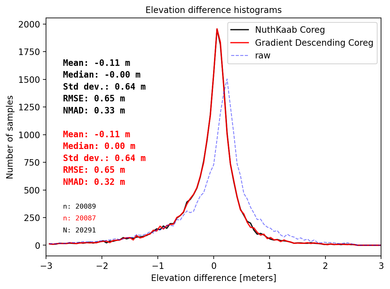
final_histogram(results_nk_10['gdf']['dh_after'],pts_10['dh'],dH_ref=results_nk_10['gdf']['dh_before'],range=(-3,3),perc_t=99.5,legend=['NuthKaab Coreg','Gradient descent Coreg','raw']);

print('NuthKaab Coreg fit matrix(e_px,n_px,bias),nmad:',results_nk_10['shift_matrix'],results_nk_10['sum']['nmad_after'])
Comparision on DTM10
Gradient descent Coreg fit matrix(e_px,n_px,bias),nmad:(-0.5000,0.3906,0.1385),0.3243
NuthKaab Coreg fit matrix(e_px,n_px,bias),nmad: (-0.47167920355557263, 0.3644381456590511, 0.137939453125) 0.32735018920898434
CPU times: total: 9.84 s
Wall time: 9.84 s
%%time

# (b) DTM 1
print('Comparision on DTM1')
## gradient descent coreg
results_1 = best_shift_px(dtm_1,sf_subset_dtm1,disp=False,stat='mix',perc_t=99.5)

## using parameters from gradient descent coreg. No bias correction.
pts_1 = get_dh_by_shift_px_gdf(dtm_1,sf_subset_dtm1,(results_1[0],results_1[1]),0,stat=False)

## plot in comparison with NuthKaab Coreg
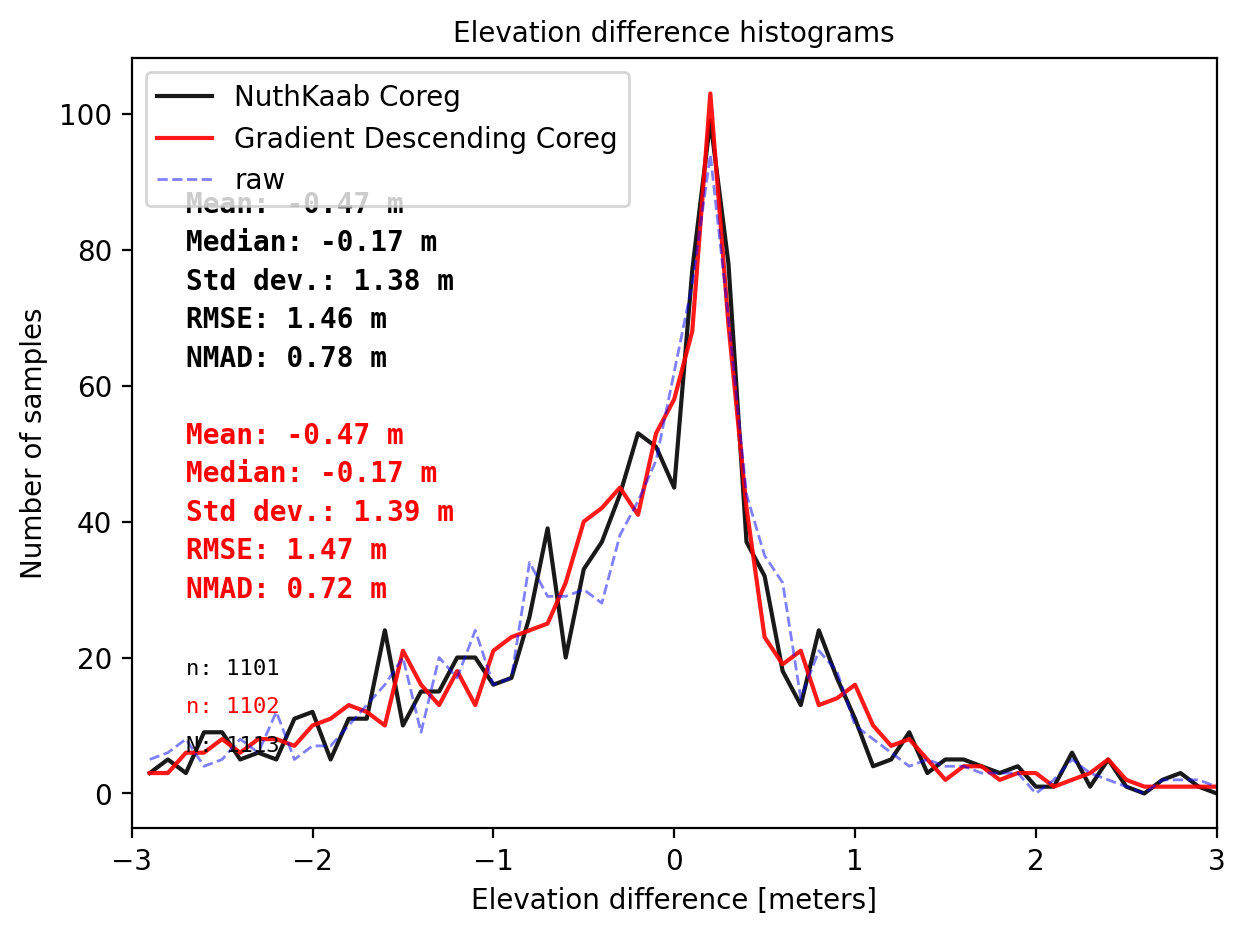
final_histogram(result_nk_1['gdf']['dh_after']+results_1[2],pts_1['dh'],dH_ref=result_nk_1['gdf']['dh_before'],range=(-3,3),bins=60,perc_t=99.5,legend=['NuthKaab Coreg','Gradient descent Coreg','raw']);

print('NuthKaab Coreg fit matrix(e_px,n_px,bias),nmad:',result_nk_1['shift_matrix'],result_nk_1['sum']['nmad_after'])
Comparision on DTM1
Gradient descent Coreg fit matrix(e_px,n_px,bias),nmad:(-0.8750,-1.2284,-0.1682),0.7210
NuthKaab Coreg fit matrix(e_px,n_px,bias),nmad: (-0.3431186328204423, -1.0512761859101158, -0.169189453125) 0.7765913818359375
CPU times: total: 641 ms
Wall time: 626 ms
%%time

# (c) DTM 1 with only 500 points

print('Comparision on DTM1 - 500 points challenge')
## gradient descent coreg
results_500 = best_shift_px(dtm_1,sf_subset_dtm1.sample(frac=1000/len(sf_subset_dtm1)),disp=False,stat='mix',perc_t=99)

## get dh using parameters from gradient descent coreg
pts_500 = get_dh_by_shift_px_gdf(dtm_1,sf_subset_dtm1,(results_500[0],results_500[1]),0,stat=False)

## plot in comparison with (b)
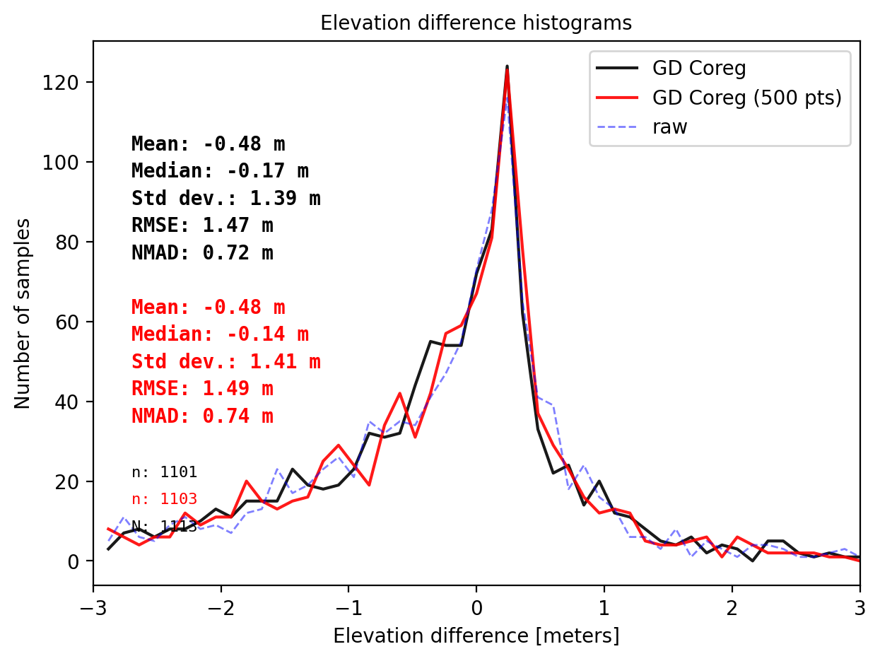
final_histogram(pts_1['dh'],pts_500['dh'],dH_ref=result_nk_1['gdf']['dh_before'],range=(-3,3),bins=50,perc_t=99.5,legend=['GD Coreg','GD Coreg (500 pts)','raw']);

print('NuthKaab Coreg fit matrix(e_px,n_px,bias),nmad: Fail to coreg')
Comparision on DTM1 - 500 points challenge
Gradient descent Coreg fit matrix(e_px,n_px,bias),nmad:(-1.0000,-0.2374,-0.1486),0.7371
NuthKaab Coreg fit matrix(e_px,n_px,bias),nmad: Fail to coreg
CPU times: total: 781 ms
Wall time: 779 ms
Section Summary
‘Gradient descent Coregistration’ is a point-based coregistration method that is significantly fast (in seconds) and efficient regardless of the resolution of the DEM. It is also able to handle datasets with a small number of points, unlike NuthKaab coregistration which requires a large sample size to work accurately.
In addition to using NMAD, my ‘Gradient descent Coregistration’ method also incorporates RMSE to make the coregistration process more ‘sensitive’ to ‘shifts’. In contrast, xDEM only uses NMAD, which may not always give the optimal offset but explained the difference in previous examples.
- However, it is important to carefully choose the hyperparameters, particularly the learning rate, to ensure that the algorithm can find the global minimum of the function.
- It is also worth noting that the results of ‘Gradient descent Coregistration’ may vary depending on the local minima reached, particularly when sample size are less than 1000 points.
- Finally, for datasets with a very large number of points (e.g. over 50000), I recommend using NuthKaab coregistration, which is very robust in these scenarios.
Not just ICESat-2
In addition to being effective for co-registering DEMs with points, ‘Gradient descent Coregistration’ also performs well for normal DEM coregistration.
To compare the speed and accuracy, we will use two different datasets: (1) a known shifted DTM10, and (2) Arctic DEM and DTM1.
- (a) xdem.NuthKaab
- (b) Gradient descent Coreg
from xsnow.godh import dem_difference_plot
from xsnow.misc import dem_shift
import xdem
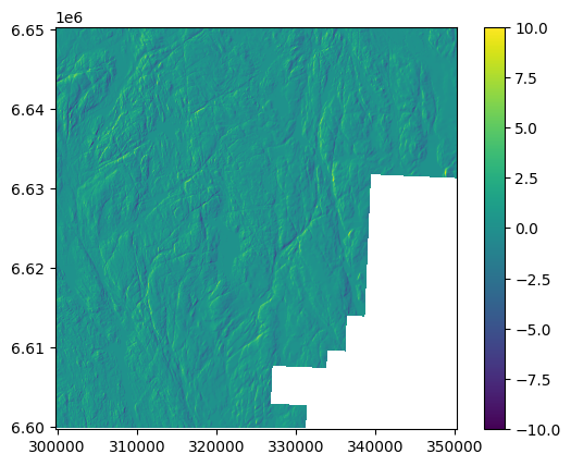
# Shift a DTM10 (1.2,-0.7) px and 0.16 m on purpose
dtm_10_shifted = dem_shift(dtm_10,1.2,-0.7,0.16)
# Plot. dh resembles to terrain.
ddem = dtm_10_shifted - dtm_10
ddem.show(vmin=-10,vmax=10)
%%time

# a. NuthKaab Coreg on DEM and shifted DEM

func = xdem.coreg.NuthKaab()
func.fit(dtm_10,dtm_10_shifted)
print(f'Coreg maxtrix east_px, north_px, bias:{func._meta["offset_east_px"]:.4f},{func._meta["offset_north_px"]:.4f},{func._meta["bias"]:.3f}')
Coreg maxtrix east_px, north_px, bias:-1.2199,0.7108,-0.160
CPU times: total: 1min
Wall time: 1min
%%time
# b. Gradient descent Coreg on DEM and shifted DEM

# sampling points from DEM
df = df_from_dem(dtm_10,samples=5000)

# runing gradient descening coreg on sampling points
best_shift_px(dtm_10_shifted,df,x0=(0,0),footprint=False,bounds=(-3,3),z_name='z',disp=False,stat='nmad',downsampling=False)
Gradient descent Coreg fit matrix(e_px,n_px,bias),nmad:(-1.1935,0.7031,-0.1600),0.0691
CPU times: total: 1.12 s
Wall time: 1.09 s


(-1.1935, 0.703125, -0.16000366, 0.06911228942871094)
The examples indicate that time reducing from 1 minutes to 1 seconds! It could be from 14 minutes to 5 seconds. Now lets looks at some real datasets. Co-registering Arctic DEM and DTM1.
## DTM1
fid_dtm1 = r'\\hypatia.uio.no\lh-mn-geofag-felles\projects\snowdepth\data\DEM\Norway\DTM1_11-11_UTM33\33-113-119.tif'
dtm1 = xdem.DEM(fid_dtm1).reproject(dst_crs=pyproj.CRS(32633),dst_res=(1,1))

grid_nn2000 = xdem.DEM('no_kv_HREF2018B_NN2000_EUREF89.tif')
dtm_1_ref = dtm1 + grid_nn2000.reproject(dtm1,resampling='bilinear')

## Arctic DEM and reproject to DTM1
fid_arctic = r'\\hypatia.uio.no\lh-mn-geofag-felles\projects\snowdepth\data\DEM\Norway\ArcticDEM\21_67_1_1_2m_v3.0\21_67_1_1_2m_v3.0_reg_dem.tif'
dtm_arctic = xdem.DEM(fid_arctic).reproject(dtm1)
%%time

# a. NuthKaab Coreg. Work on 1m resolution.

func = xdem.coreg.NuthKaab()
func.fit(dtm_1_ref,dtm_arctic)
print(f'Coreg maxtrix east_px, north_px, bias:{func._meta["offset_east_px"]:.4f},{func._meta["offset_north_px"]:.4f},{func._meta["bias"]:.3f}')
Coreg maxtrix east_px, north_px, bias:5.1641,-4.1300,-0.555
CPU times: total: 14min 4s
Wall time: 14min 4s
%%time
# b. Gradient descent Coreg. Work on 1m resolution.

# sampling points from DEM_Ref
df_ref = df_from_dem(dtm_1_ref,samples=10000)

# runing gradient descening coreg on sampling points
res_gd =best_shift_px(dtm_arctic,df_ref,x0=(0,0),footprint=False,bounds=(-5,5),z_name='z',disp=False,stat='mix',downsampling=False,perc_t=99)
Gradient descent Coreg fit matrix(e_px,n_px,bias),nmad:(2.7500,-3.4922,-0.5269),0.9925
CPU times: total: 5.25 s
Wall time: 5.25 s
import matplotlib.pyplot as plt
# ddem
ddem_raw = dtm_arctic - dtm_1_ref
ddem_coreg_nuthkaab = dem_shift(dtm_arctic,5.1641,-4.13,-0.555) - dtm_1_ref
ddem_coreg_gd = dem_shift(dtm_arctic,2.7500,-3.4922,-0.5269) - dtm_1_ref

# plot
fig, (ax1,ax2,ax3) = plt.subplots(1,3, figsize=(18, 6))

ddem_coreg_nuthkaab.show(ax=ax1, vmax=2,vmin=-2,cb_title='dH (m)')
ddem_coreg_gd.show(ax=ax2, vmax=2,vmin=-2)

ax1.set_title('dH (coreg_nuthkaab)')
ax2.set_title('dH (coreg_gradient_descent)')
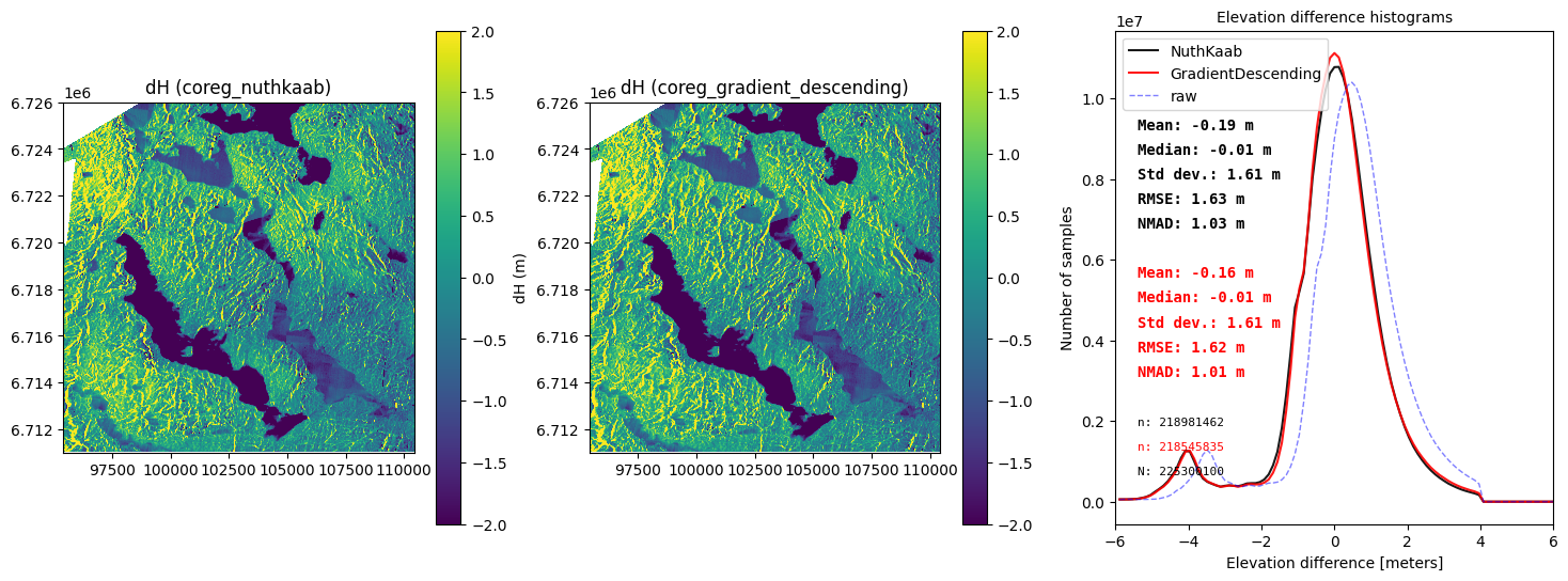
final_histogram(ddem_coreg_nuthkaab,ddem_coreg_gd,dH_ref=ddem_raw,range=(-6,6),ax=ax3,legend=['NuthKaab','Gradientdescent','raw'])
Section Summary
Arctic DEM in this area (close to Finse) is a snow-on DEM. So, there is no reason to do bias correction e.g. -0.555 m or -0.5269 m (This is snow depth over the entire area acrtually). For the same reason, snow cover introduce errors that make it challenging to obtain reliable co-registration results. In this competition.
- NuthKaab give a shift matrix (5.1641,-4.13) with NMAD 1.03 m in 14 minutes
- Gradiant descent Corg give a shift matrix (2.7500,-3.4922) with NMAD 1.01 m in just 5 seconds.
Based on these results, we conclude that ‘Gradient descent Coregistration’ is the superior method in all scenarios. Additionally, ‘Gradient descent Coregistration’ can easily support rotation correction, making it even more versatile.
Point Interpolation Vs Zonal Statistics of the Footprint
When picking up a value at a point on a DEM, the value may not match the grid exactly and instead is an interpolated value.
In xDEM, interpolation is implemented using scipy.ndimapge.map_coordinates, which supports nearest, bilinear, and bicubic interpolation. Bicubic interpolation is sometimes better than bilinear interpolation, but this is not always the case.
Another option for evaluating the value at a point on a DEM is to use zonal statistics, which calculates a statistic (e.g. mean, median, etc.) for the area surrounding the point. This can be particularly useful for high-resolution DEMs, where the statistic value of the footprint may provide a more accurate representation of the true value because the statistics removed the noisy spikes.
So, What is the best footprint size for zonal statistics? Again, I used gradient descent to find it!
I will use DTM1 and ICESat-2 snow-free measurements as an example to demonstrate the difference of two methods.
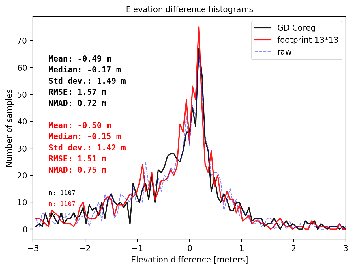
# The footprint of ICESat-2 is about 13 m by 13 m.
pts_size = get_dh_by_footprint(dtm_1, sf_subset_dtm1,(13,13),z_name='h_te_best_fit',s_name='mean',stat=None,perc_t=99.75)

## plot
final_histogram(pts_1['dh'],pts_size['dh'],dH_ref=result_nk_1['gdf']['dh_before'],range=(-3,3),perc_t=99.75,legend=['GD Coreg','footprint 13*13','raw']);
# Gradient descent suggest the better size
size = best_footprint(dtm_1, sf_subset_dtm1,(13,13),z_name='h_te_best_fit',s_name='mean',stat='mix',perc_t=99.75)
the best fit footprint(width,length): (8.0000,25.1250)
# Use the 'best' size to get elevation difference
pts_size = get_dh_by_footprint(dtm_1, sf_subset_dtm1,(8,25.125),z_name='h_te_best_fit',s_name='mean',stat=None,perc_t=99.75)

## plot
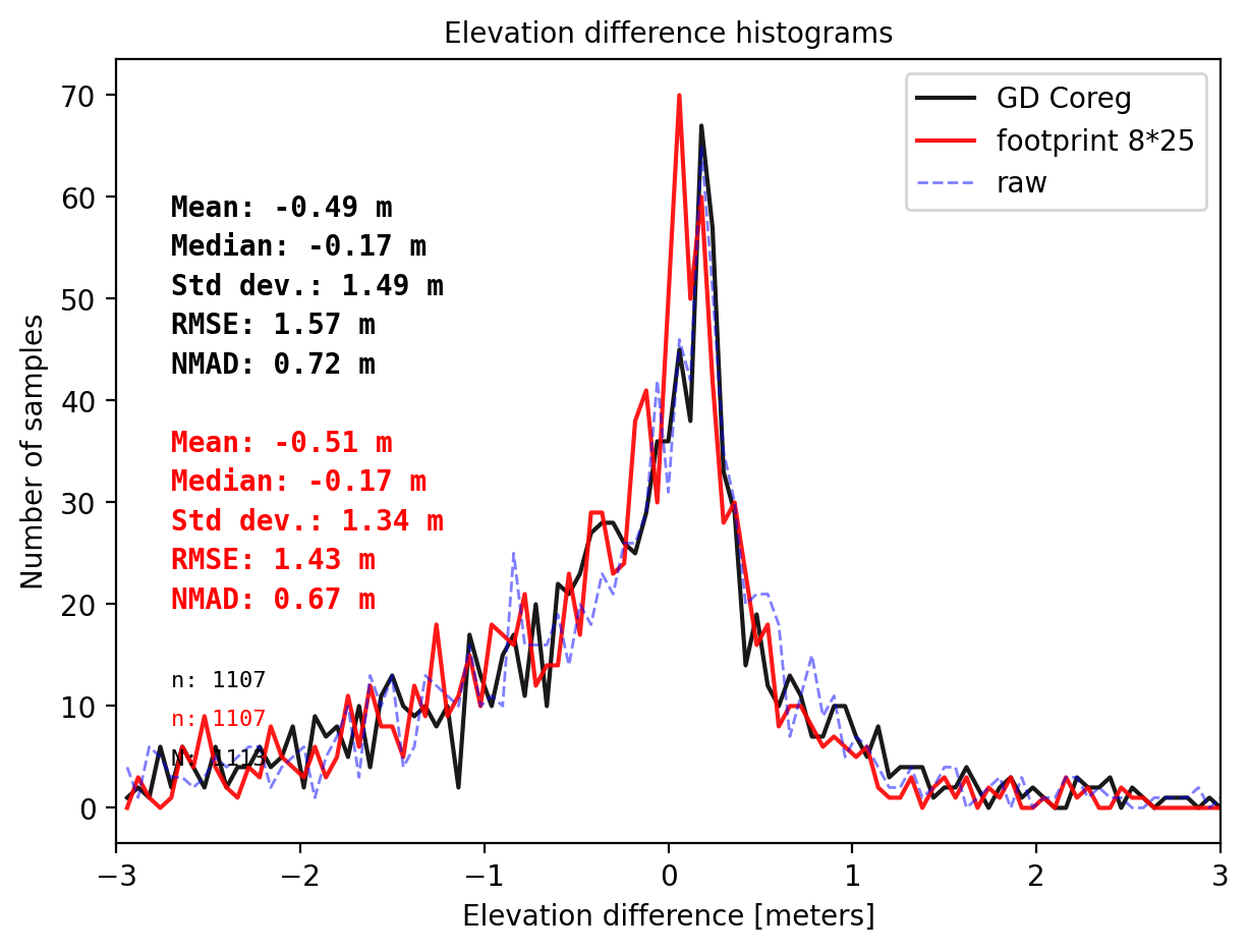
final_histogram(pts_1['dh'],pts_size['dh'],dH_ref=result_nk_1['gdf']['dh_before'],range=(-3,3),perc_t=99.75,legend=['GD Coreg','footprint 8*25','raw']);
# Use the size to get elevation difference
pts_13100 = get_dh_by_footprint(dtm_1, sf_subset_dtm1,(13,100),z_name='h_te_best_fit',s_name='mean',stat=None,perc_t=99.75)

## plot
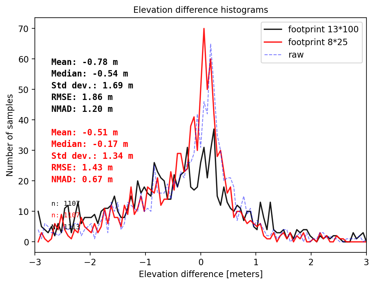
final_histogram(pts_13100['dh'],pts_size['dh'],dH_ref=result_nk_1['gdf']['dh_before'],range=(-3,3),perc_t=99.75,legend=['footprint 13*100','footprint 8*25','raw']);
Section Summary
It is controversial to decide which one to use, point interpolation (with coreg) or footprint zonal statistics. So far we have matched ICESat-2 ‘s h_te_bestfit with values from:
- interpolation (and coreg) with NMAD 0.72 m.
- foorprint 13x13 m with NMAD 0.75 m (the footprint size naturally)
- foorprint 8x25 m with NMAD 0.67 m (the best footprint suggest by gradient descent algorithm)
- foorprint 13x100 m with NMAD 1.20 m (the footprint size of ATL08 segment)
However, the results are hard to be reliable due to the small sample size. But gradient descent is very useful for applications on DEM or ICESat-2 dataset.