What if the ice block expedition 1959 happens in 2021?
You cannot blame it to climate change
A million tons of ice was shipped from Norway each year during the golden age of ice trade to England, India, South America, China and Australia. The business that involved transporting natural ice for commercial purposes started at 1806, flourished in the end of 19th-century and was replaced by plant ice until World War I (“Ice Trade,” 2022). A primary concern of the ice transportation is the melt loss.
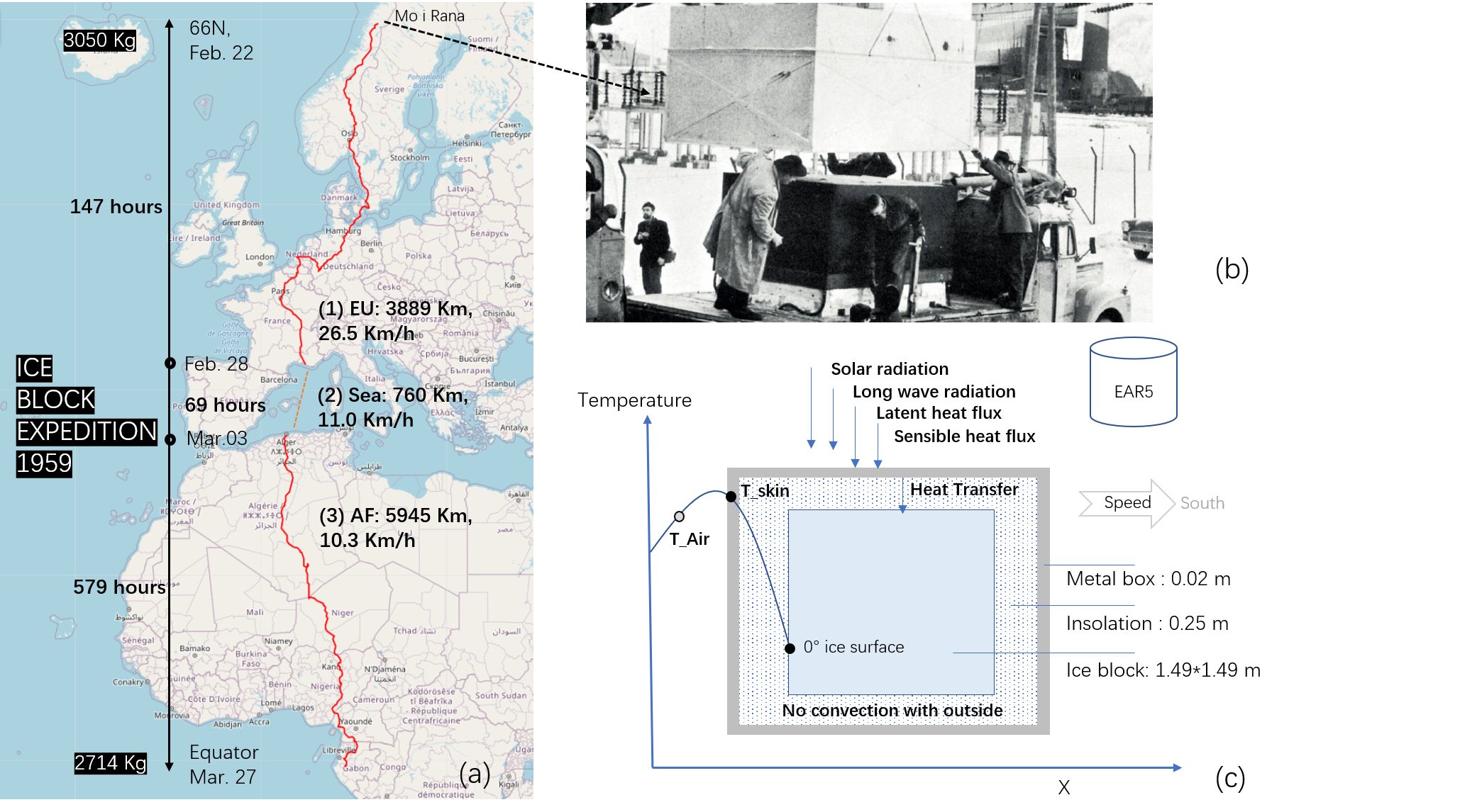
Luckily, there is a record to follow. In 1959, a three-ton block of ice from Mo i Rana by the Arctic Circle was trucked to Libreville by the Equator in an advertisement of insulation materials. The event left enough details and measurements: 2714 Kg ice remained with only 11% mass loss(“Ice Block Expedition of 1959,” 2022) in a 37 day long journey.
Using the EAR5 climate reanalysis dataset (Muñoz Sabater, 2021), this study is able to simulate the 1959 ice block expedition by surface energy balance equations and heat transfer equations, which is a new perspective on this event and the topic of ice trade.
Solutions
- The physics basis:
- Surface energy balance
- Heat equation
- Wind log profile
- Total heat resistance
- Dataset:
- The requirements:
- numpy, pandas
- [process kml] geopandas, shapely
- [heat equations] numba, scipy
Please find the solutions from liuh886/the_ice_block_expedition_1959: Simulate the ice block expedition1959 by energy balance equations and heat equations (github.com) .
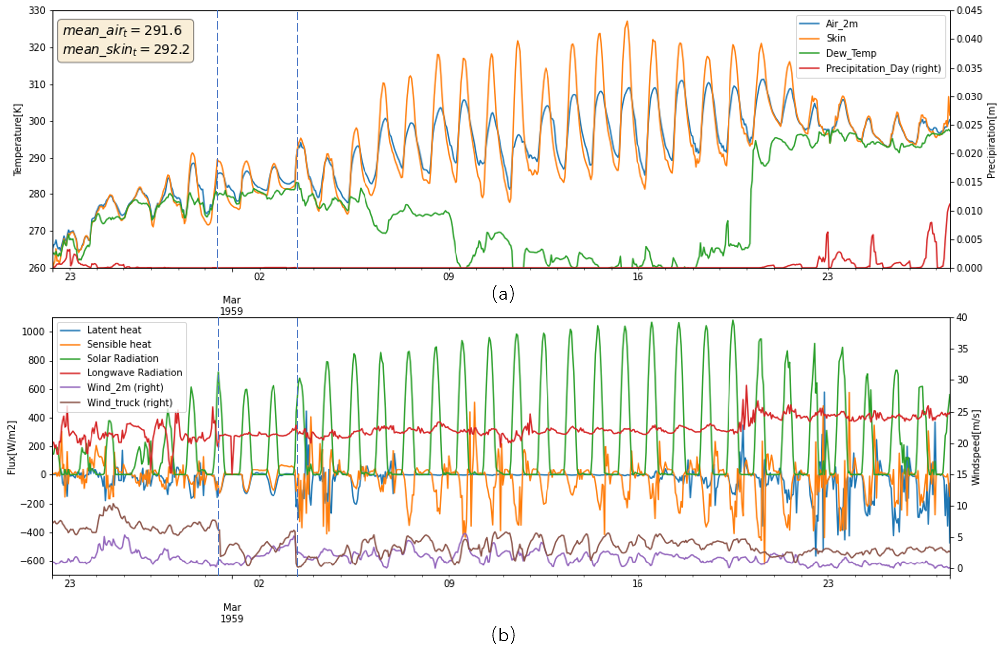
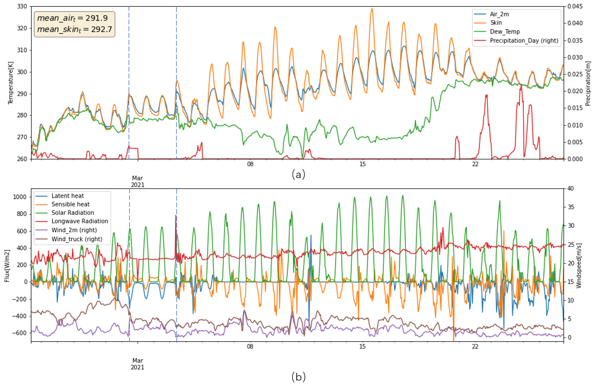
Weather - 1959 vs 2021
Scenario - Bare ice
What if the expedition went with an ice block without any protection?
Scenario - 1959, 2021 and the original records
In original records, only four liters of water had been shed when the truck arrived in Algiers on 3th March 1959. When crossing the Sahara, on average 15 liters melted each day. Finally, only 336 kg ice lost in end of expedition, which is 11.0% of the total mass.
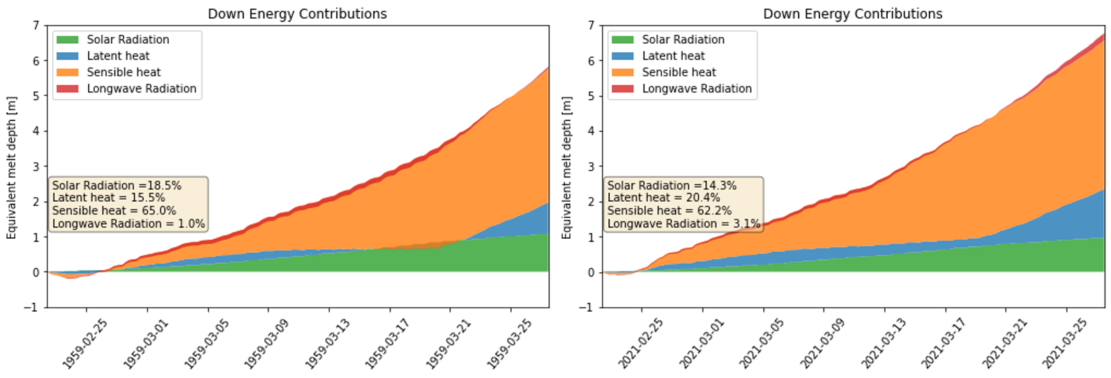
In the simulations, Figure below displays that ice mass loss of 352.3 Kg and 348.2 Kg in 1959 and 2021, with 322.8 Kg in 2020 as a reference, which is opposite to the scenario of bare ice. In ice without cover scenario, the bare ice in 2021 melt more than 1959 due to higher air temperature, and more contributions from latent heat and longwave radiation. However, if there is a cover upon ice, the melt mechanism would be different, because the cover does not have phase change. Thus, the longwave radiation and sensible heat actually are going to be cooling component not the melt energy component when it is warmer than air temperature. If water is available, the evaporation would take heat away as well.
Table shows that, in the scenario of aluminum_glasswool_1959, the mass loss is 26.5 Kg until Algiers, 14.3 Kg per day in desert, 352.3 Kg in the final destination, which are slightly different with the original records.
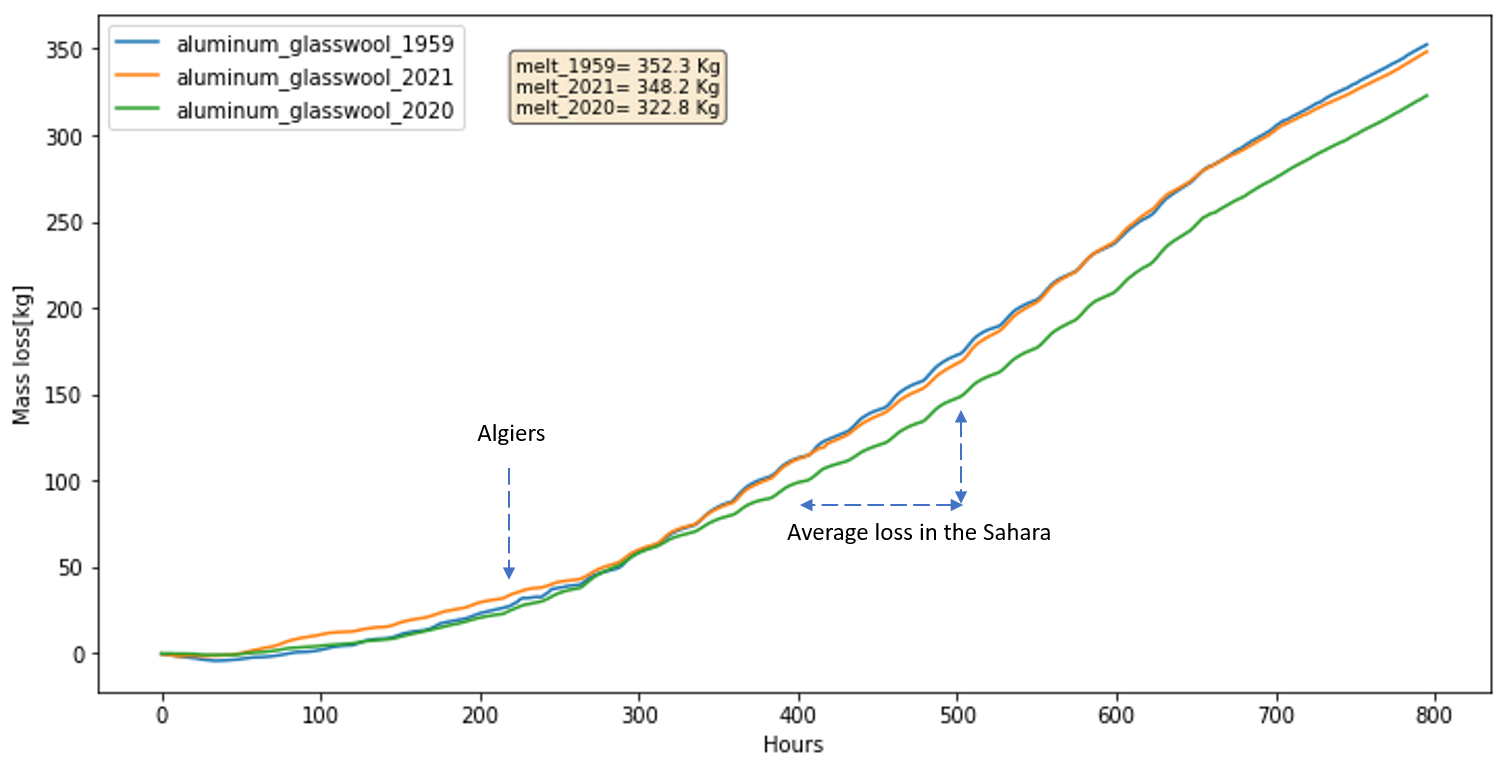
Table. The scenario - 1959, 2021 and the original records
| Event | Initial Mass [Kg] | Insulation | Insulation thickness[m] | Mass lost Algiers [Kg] | Mass loss Sahara [Kg/day] | Mass loss In total [Kg] |
|---|---|---|---|---|---|---|
| Original records | 3050 | Mainly glass wool | - | About 4 | About 15 | 336 |
| Aluminum_glasswool_1959 | 3050 | Glass wool | 0.25 | 26.5 | 14.3 | 352.3 |
| Aluminum_glasswool_2021 | 3050 | Glass wool | 0.25 | 32.0 | 13.2 | 348.2 |
| Aluminum_glasswool_2020 | 3050 | Glass wool | 0.25 | 23.0 | 11.7 | 322.8 |
Heat equation model
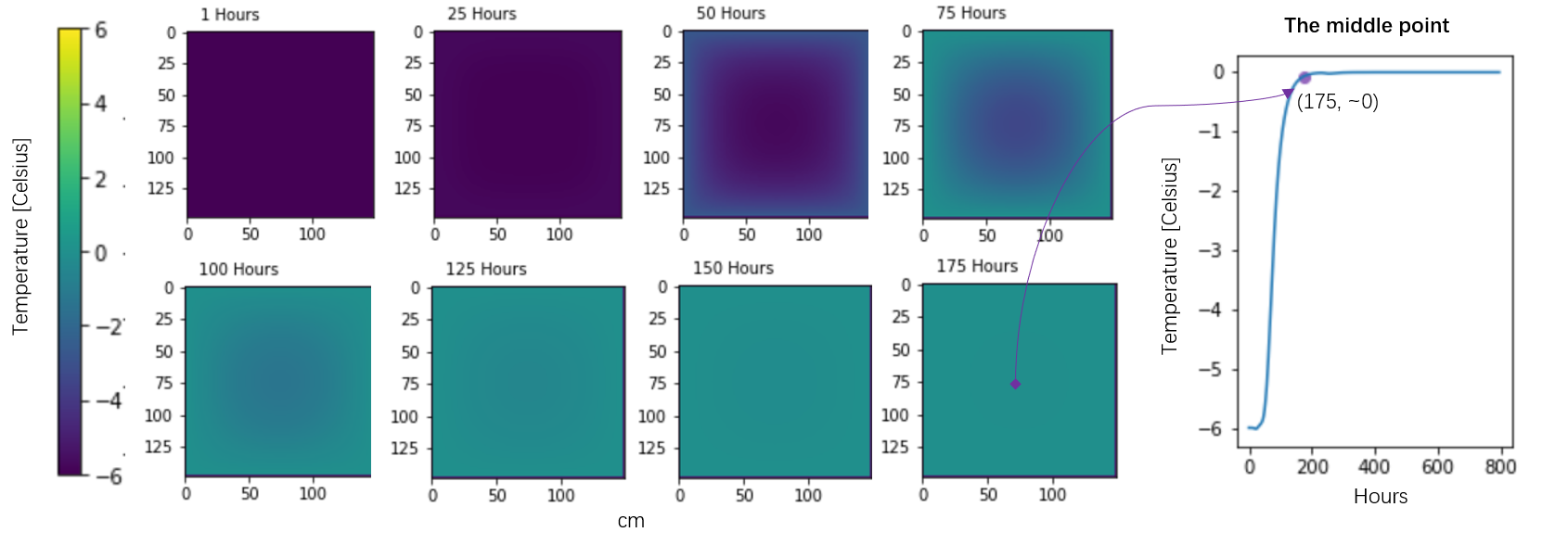
The surface energy balance model can only give the amount of heat transfer, which is assumed to be melt energy. But the real changes within the box are still unknow, e.g. (1) What is the temperature distribution of the ice block, or how does the temperature of the ice core fluctuate? (2) How long does it take for ice to melt after warming up to 0 degree Celsius.
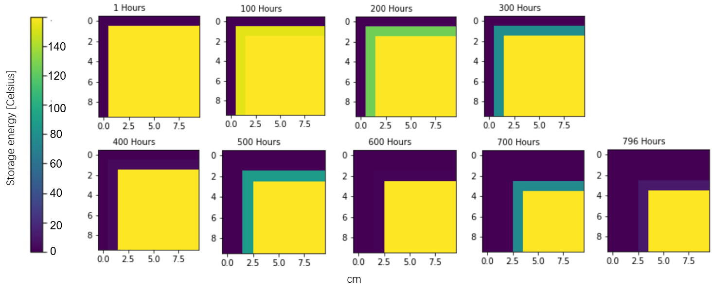
The first layer is equal to 122.1 Kg, the second is 118.9 Kg. The third layer is 115.7 Kg, but it does not go completely. The remain storage energy in temperature is 10.8 K. So, a rough estimation is the (1-10/158.4) *115.7 = 107.8 Kg. Then, the accumulative mass loss is 348.8 Kg.
Key codes
def q_latent(air_pressure,air_temp_K,wind_2,es,ea): # downward positive

    # calculate latent heat # ASSUME: water is always available! satuation = 1
    # input:
    # - es, ea, air_pressure  in Pa
    # - air_temp_K in K
    # - wind_2 in m/s
    # output:
    # - q_lat in W/m-2

    rho_air = air_pressure/(287.058*air_temp_K)  # air density [kg /m^3], T in K
    lv = (2500.8-2.36*(air_temp_K-273.15))*1000; #latent heat of evaporation of water [J/kg], T in C
    A = 0.4*0.4 / np.log(2/1e-2) / np.log(2/1e-2) # k = 0.4

    q_lat = -0.622*rho_air*lv*A*wind_2*(es-ea)/air_pressure; # potential evaporation ASSUME: water is available

    return q_lat

def q_sensi(air_pressure,air_temp_K,wind_2,ta,ts): # downward positive
    # calculate sensible heat
    # input:
    # - ta, ts in same unit, K or T
    # - air_temp_K in K
    # - wind_2 in m/s
    # output:
    # - q_sen in W/m-2
    cp_air = 1005  # heat capacity of air   J/(kg*K)

    rho_air = air_pressure/(287.058*air_temp_K)  # air density [kg /m^3], T in K
    lv = (2500.8-2.36*(air_temp_K-273.15))*1000; #latent heat of evaporation of water [J/kg], T in C
    A = 0.4*0.4 / np.log(2/1e-2) / np.log(2/1e-2) # k = 0.4

    q_sen = cp_air*rho_air*A*wind_2*(ta-ts)
    return q_sen

## 2d heat equation

import copy
from numba import jit
import numpy as np
from scipy.ndimage import binary_dilation, binary_erosion

# 1 environment
box_t = np.loadtxt('1959_box_temp.csv')

# 2 settings
a_ice = 1.19e-6 # heat difussivity [m2/s]
a_air = 18.46e-6 # heat difussivity [m2/s]
a_gw = 1.785e-6 # heat difussivity [m2/s]

lf = 334000 #Latent heat of fusion L f = 334 000 J/kg -1 (phase change ice – water)
cp_ice = 2108 # J/(kgK)
rho_ice = 917 # Kg/m3

t_ice = -6 # initial temperature of ice
dx=0.01 # 1cm nodes
dt = 1 # seconds
hours = len(box_t) # hours here is 796
# 3 initial
heatmap = np.zeros([ice_width,ice_width])+t_ice # inital temp
block = np.ones([ice_width,ice_width])   # initial musk   1:ice 0:air
tt = lf*rho_ice*0.01*0.01*0.01/(cp_ice*rho_ice*0.01*0.01*0.01)-t_ice  # energy musk: the energy required to melt in [K]
energy = block*tt

block[[0,-1],:]=0 # air boundary
block[:,[0,-1]]=0

energy[[0,-1],:]=0 # air boundary
energy[:,[0,-1]]=0

@jit(nopython=True, nogil=True)
def iteration(cs,inner_musk,energy,outer_musk,box_t):
    ns = cs.copy() # new state
    ns_energy = energy.copy() # new state
    ly,lx = ns.shape
    for i in range(0,lx):
        for j in range(0,ly):
            if outer_musk[j][i] == 1: #outer node
                #heat flux -> warm-up
                #q = (box_t-cs[j][i])/0.25*0.04   # W/m2
                #dT = q/(917*0.01)/2108
                ns[j][i] = cs[j][i] +  (box_t-cs[j][i])/0.25*0.04/(917*0.01)/2108*dt
                ns_energy[j][i] = energy[j][i] - (box_t-cs[j][i])/0.25*0.04/(917*0.01)/2108*dt
                #ns_energy[j][i] = energy[j][i] - 30/3600*dt

                # ->add energy storage -> latent heat flux
                if ns[j][i]>0:
                    ns[j][i] = 0

            if inner_musk[j][i] == 1: #inner node
                ns[j][i] = cs[j][i] + a_ice*dt/dx**2 * (cs[j+1][i] + cs[j-1][i] +
                                                        cs[j][i+1]+cs[j][i-1]-
                                                        4*cs[j][i])
            else: #pass boundry conditon
                pass
    return ns,ns_energy
def find_outer_musk(a):
    a= a.astype(int)
    k = np.ones((3,3),dtype=int) # for 4-connected
    #k = np.zeros((3,3),dtype=int); k[1] = 1; k[:,1] = 1 # for 8-connected
    out = binary_dilation(a==0, k) & a
    inside = binary_erosion(a).astype(a.dtype)
    return out,inside

def solve_heat(heatmap,block,box_temp_list,energy):
    hm_list = []
    block_list = []
    energy_list = []
    inner_musk_list = []
    cs = heatmap.copy() # initial temp state
    energy_musk = energy.copy()
    block_musk = block.copy()

    for h in range(0,hours):

        for t in range(1,3600): # iteration in seconds
            # HEAT diffusion
            outer_musk,inner_musk = find_outer_musk(block_musk)
            cs,energy_musk = iteration(cs,inner_musk,energy_musk,outer_musk,box_temp_list[h]) #update cs and energy_musk
            block_musk[energy_musk <0] = 0 # update blockmusk: TURN INTO AIR
        if h%1 ==0: # return every hour
            hm_list.append(cs)
            block_list.append(block_musk.copy())
            energy_list.append(energy_musk)
            inner_musk_list.append(inner_musk)
            print('Now: in hour',len(hm_list))
    return hm_list,block_list,energy_list,inner_musk_list

### Main

hm_list_2d,block_2d,energy_2d,inner_musk_2d = solve_heat(heatmap,block,box_t,energy)
Few thoughts
1D Surface energy balance equations are used on the control surface. And the heat equations can be applied to 2D or 3D homogeneous material.
There are some results that are very close the original records. The simulations show that only about 3 cm thick, or 348.8 Kg to 352.3 Kg of the ice block melted. The heat equation simulation revealed temperature distribution of ice inside the box. The ice block takes 175 hours warming up from -6° to 0° in the expedition.
Transporting ice to the tropics in the 19th century was totally manageable business. Using a white-covered wooden box filled with double thickness is able to achieve the same insulation effect as glass wool, which is fully expected by simulations. We can use the ice block expedition of 1959 as a baseline. If we do an expedition again, the melt loss of transporting ice is not expected over than 1959. And, the simulations do not support blaming it to climate change because there is a covering upon ice.
The simulations could also explain the role of debris cover on glacier ablation.