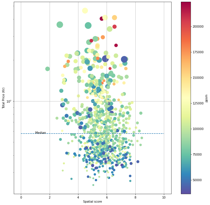
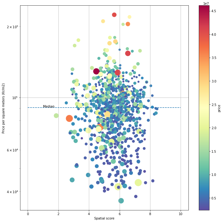
Using 5.8 million to buy a unit in Oslo, which one is worth?
Housing Price MCDA Model - a perspective from spatial contributions
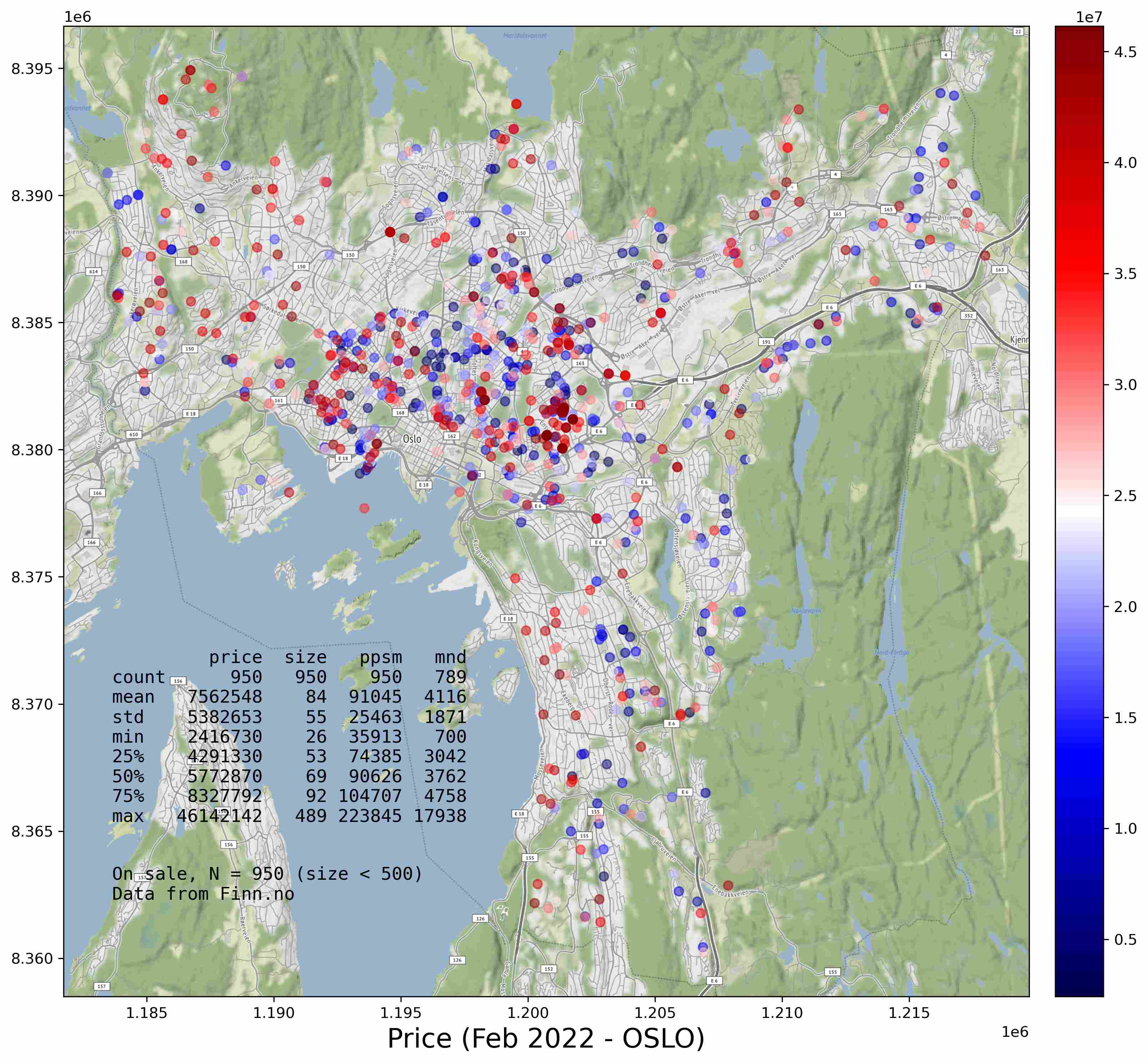
There are so many factors contributing to house prices. At the same location, the price varies by building’s attributes, e.g., the cost of construction, design, decoration, and furnishings. If a pair of twin buildings exist, which are at different locations, the surrounding environment will decide price. In this report, we defined surroundings as spatial contributions or spatial `scores.
Some like to live in the city center, enjoying night pubs, and shopping malls, whereas others prefer being near the forest. So, the unit’s price or value varies from different perspectives. Multi-criterion decision analysis (MCDA) is to support decision-makers in solving such problems (Meng et al., 2011; “Multiple-Criteria Decision Analysis,” 2022).**
This report proposed a Housing Price MCDA Model (HPMM) to value the spatial contributions by inputting user preferences, based on spatial information from open access databases (Norwegian Public Roads Administration, Statistics Norway), OpenStreetMap, and satellite images. The model is aimed to provide best-fitting options for house **buyers and **assessing the living** conditions in various areas of Oslo for better urban planning regulation**. In the end, I discussed the weakness of the model, and the several shopping tips revealed by the model.
This is a demonstration model that could be extended to other cities easily. The post-processed datasets in this project are good materials for automating GIS or WebGIS training courses. However, I had no time to make this model online due to limited time.
How it works
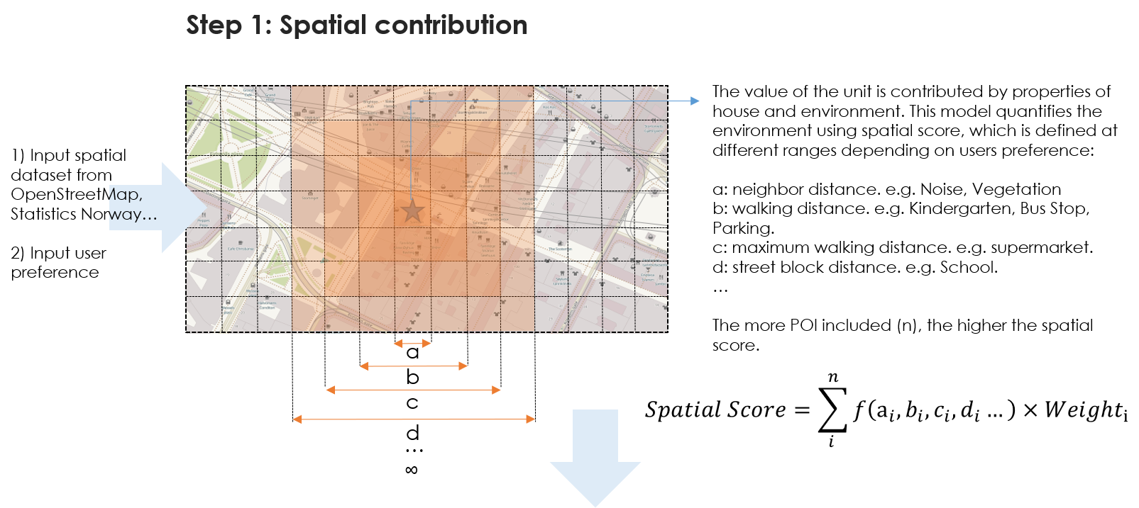
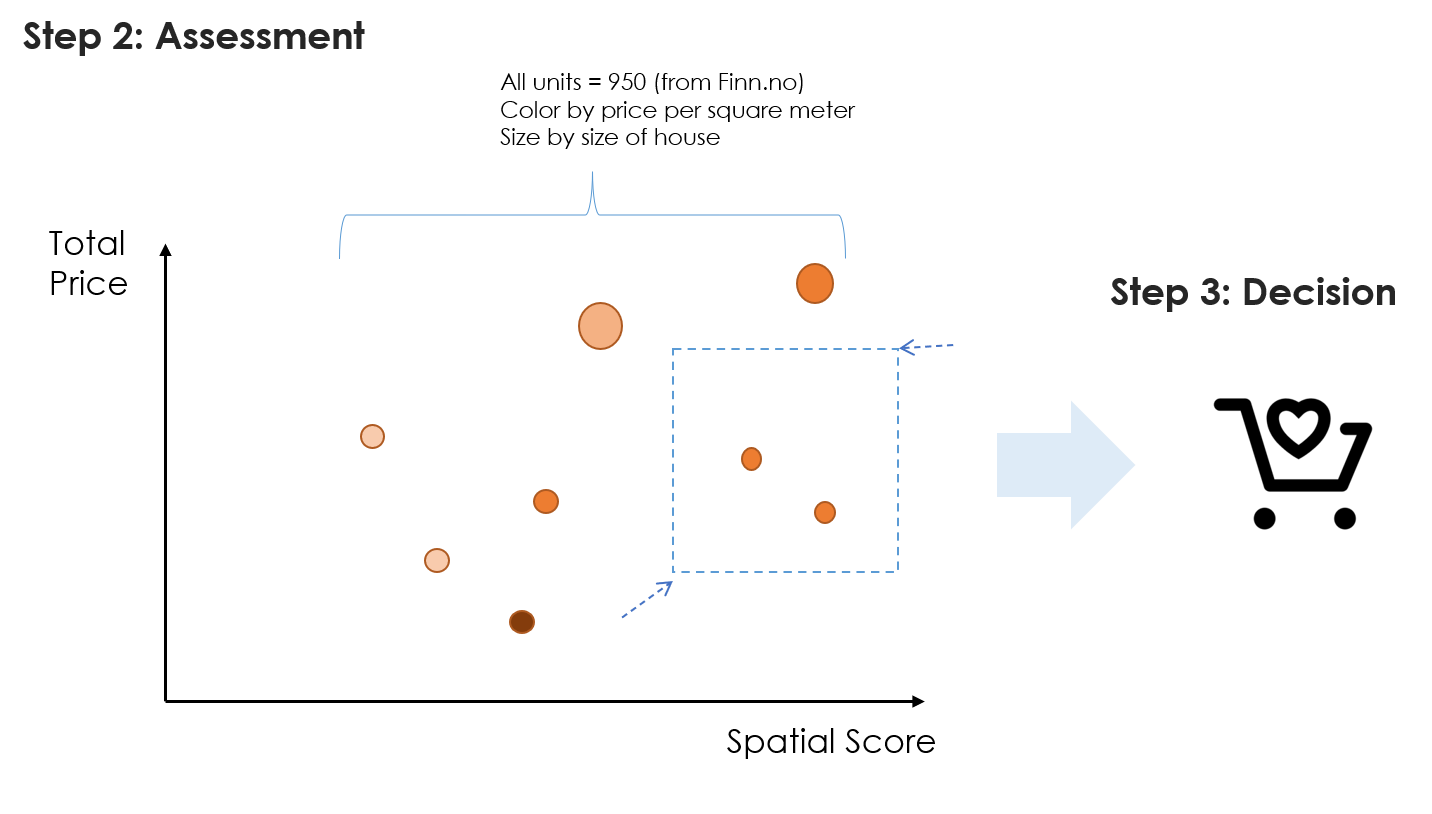
HPMM obtains (1) spatial information from statistics Norway, OpenStreetMap and optical satellite imagery, (2) user preferences, including point of interest (POI) and weights for all criteria. Once the model is set up, the on-sale units of Oslo in February from Finn.no are inputted to model. Then, the recommended units are output by model.
Oslo County polygon was resampled into a 50x50 meters grid first. All spatial information was accordingly assigned into each cell by location. The spatial information used in this scenario includes public transportation, kindergarten, school, stores, groceries, culture and sports building, parking places, vegetation index, and noise level. The spatial score is contributed by all these elements i on different distance a/b/c/d… and weights under certain reclassifying rules f(x).
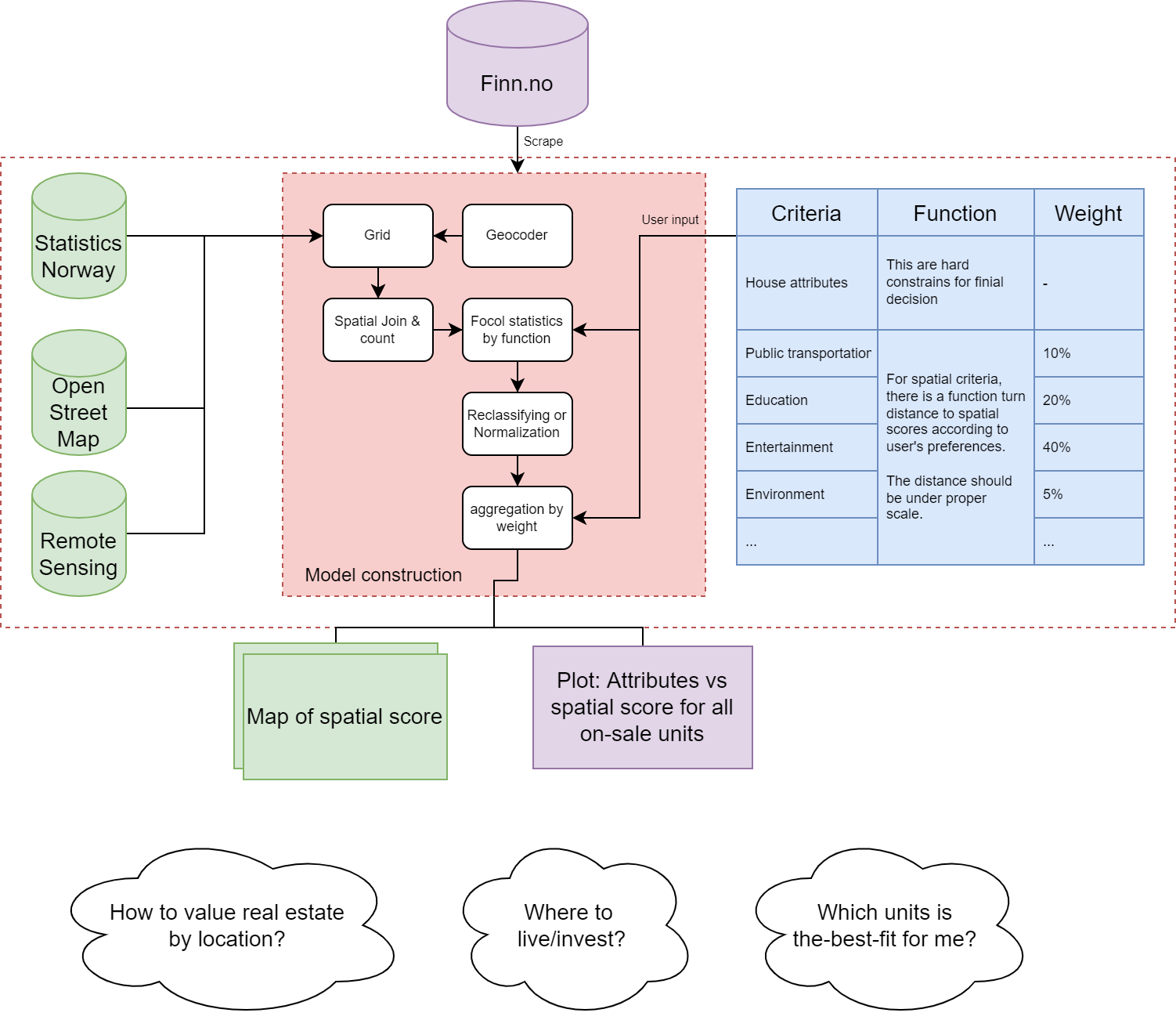
The main tools used in this project:
- Scraping data from Finn by scrapy/scrapy: Scrapy, a fast high-level web crawling & scraping framework for Python. (github.com)
- Geocoder from GeoPy).
- Spatial joining, calculation, cleaning, and visualizing by GeoPandas
- Focal statistics, reclassification, raster calculator, extract multi values to points by ArcGIS Pro.
The parameters used in the demo model: Table 1. The criteria and the model parameters (demo).
| Code | Criteria | Type | Spatial points by function | Reclassifying | Weight |
|---|---|---|---|---|---|
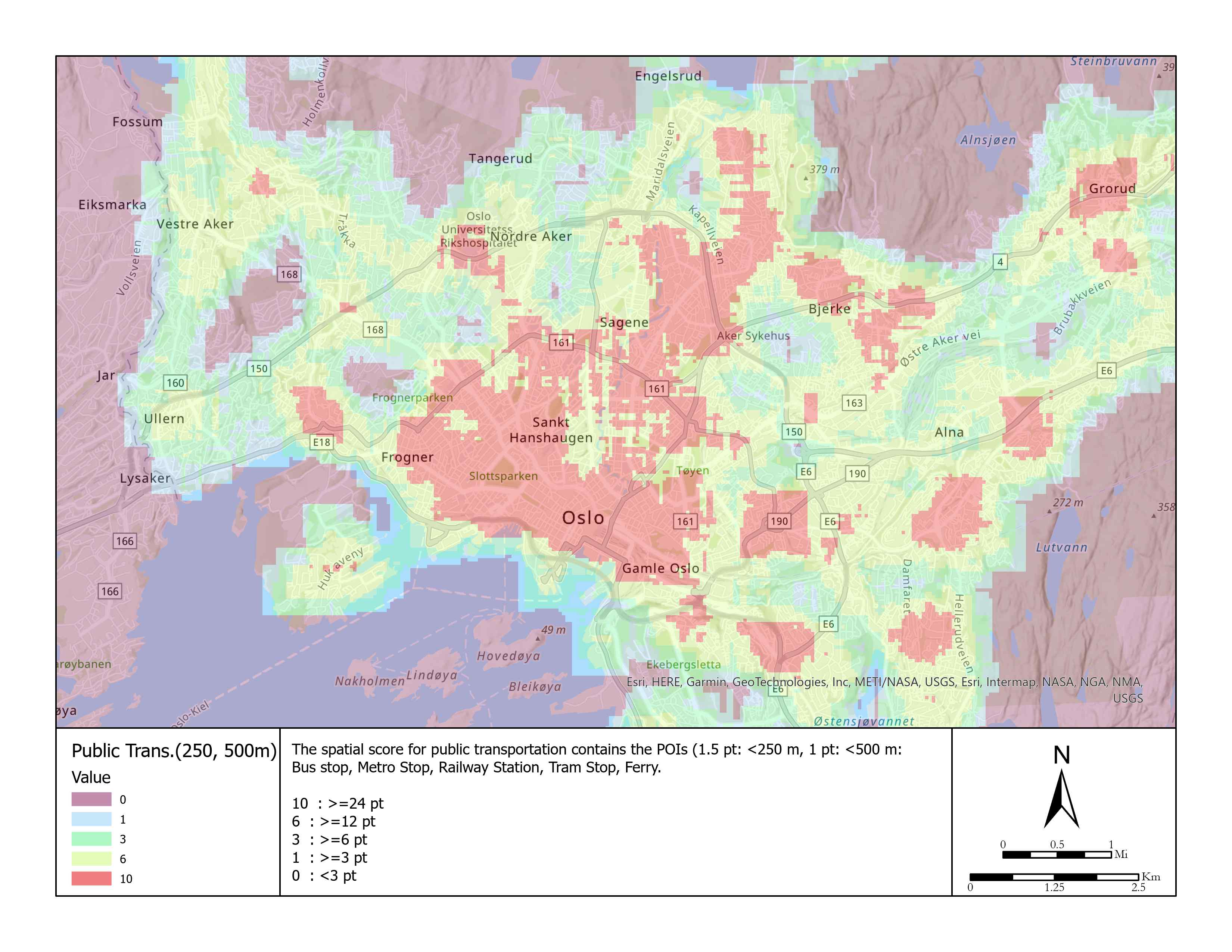
| 1 | Bus or metro Stop | Numerical | 1.5 pt: <250 m 1 pt: <500 m 0 pt: >=500 m | 10 pt : >=24 pt 6 pt : >=12 pt 3pt : >=6 pt 1 pt : >=3 pt 0 pt : <3 pt | 15 |
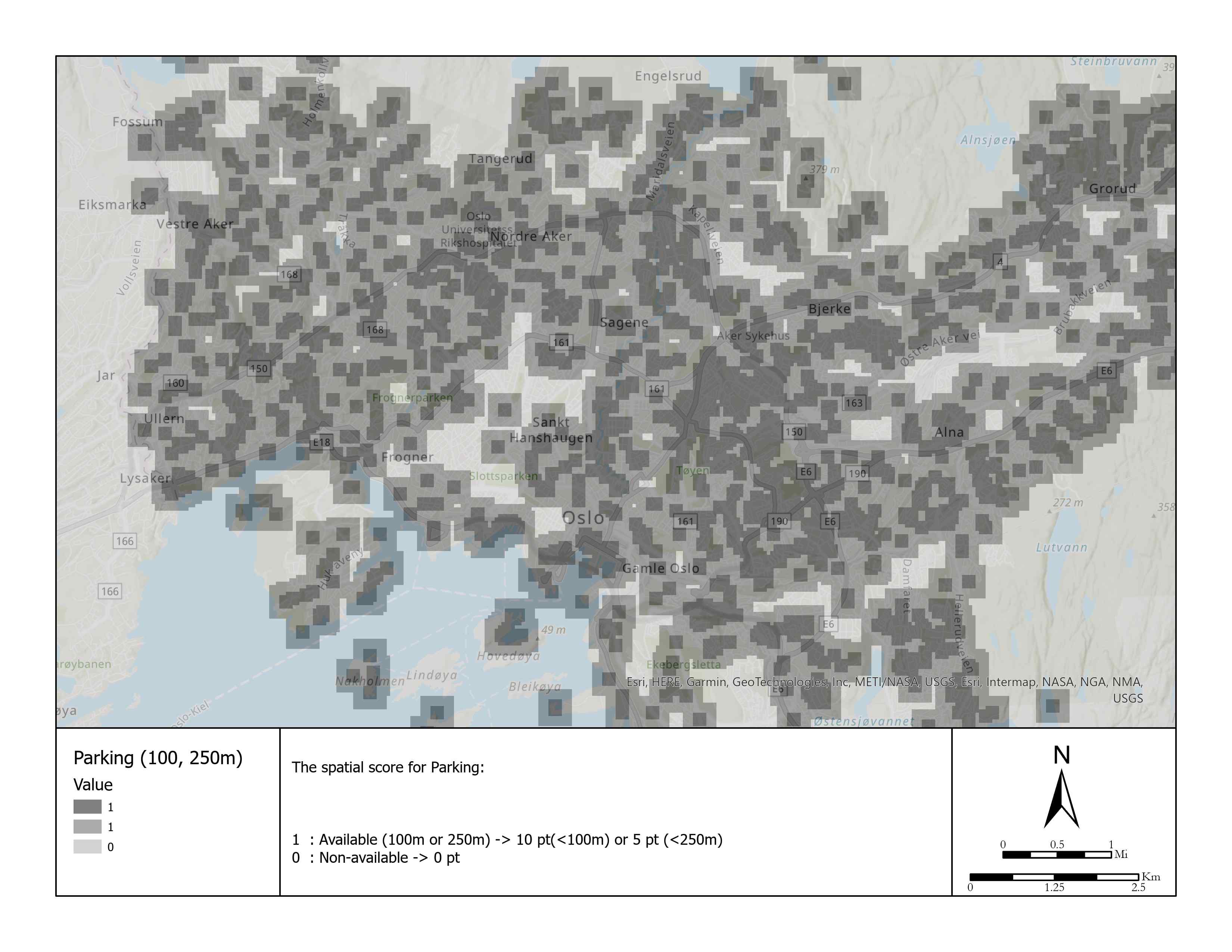
| 2 | Parking place | Boolean | 10 pt: =<100 m 5 pt: =<250 m 0 pt: >=250 m | - | 5 |
| 3 | Kindergarten | Boolean | 10 pt: <500 m 0 pt: >=500 m | - | 10 |
| 4 | School | Boolean | 10 pt: <500 m 0 pt: >=500 m | - | 5 |
| 5 | Supermarket | Boolean | 10 pt: <250 m 5 pt: <500 m 0 pt: >=500 m | - | 10 |
| 6 | Café, Bakery, Bar, Restaurant, Pharmacy, Fast food, Convenience store, Beverage | Numerical | 1 pt: <500 m 0 pt: >=500 m | 10 pt : >=50 pt 8 pt : >=25 pt 6pt : >=8 pt 4 pt : >=4 pt 0 pt : <4 pt | 5 |
| 7 | Library, Museum, Theatre, Stadium, Sports center, Cinema, Playground, Mall, Swimming pool | Numerical | 1 pt: <500 m 0 pt: >=500 m | 10 pt : >=15 pt 6 pt : >=8 pt 3pt : >=3 pt 1 pt : >=1 pt 0 pt : <1 pt | 5 |
| 8 | College, University, Hospital | Numerical | 1 pt: <1000 m 0 pt: >=1000 m | 10 pt : >=7 pt 5 pt: >=4 pt 1 pt: >=1 pt 0 pt : <1 pt | 5 |
| 9 | NDVI | Numerical | Average of 50 m | 10 pt: 70% 6 pt: 50% 4 pt: 30% 0 pt: below 30% | 20 |
| 10 | Noise | Numerical | Average of 50 m | 10 pt: <= 55db 2 pt: <= 60db 1 pt: <= 65db 0 pt: >65db | 20 |
Some results
Taking public transportation or driving? Or half-half.
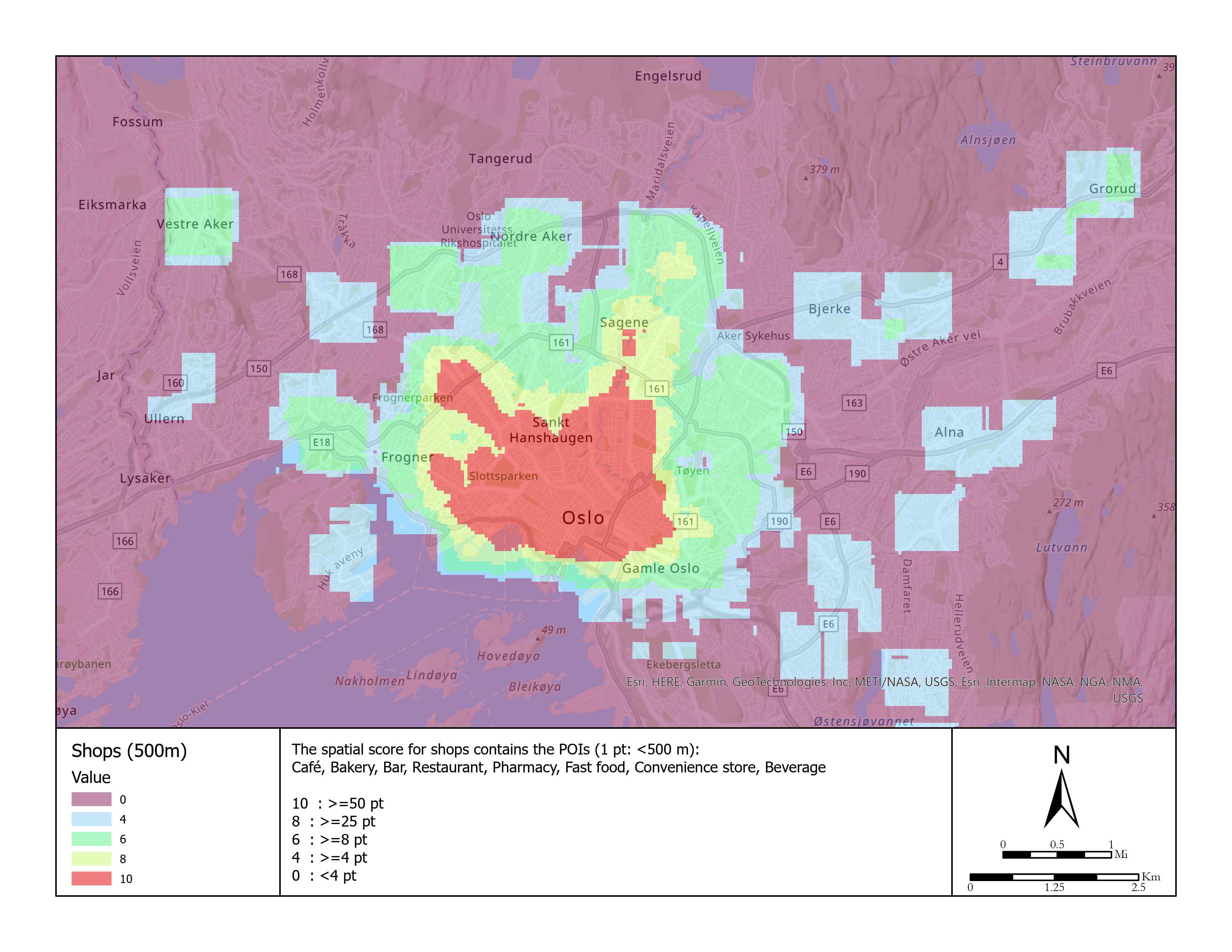
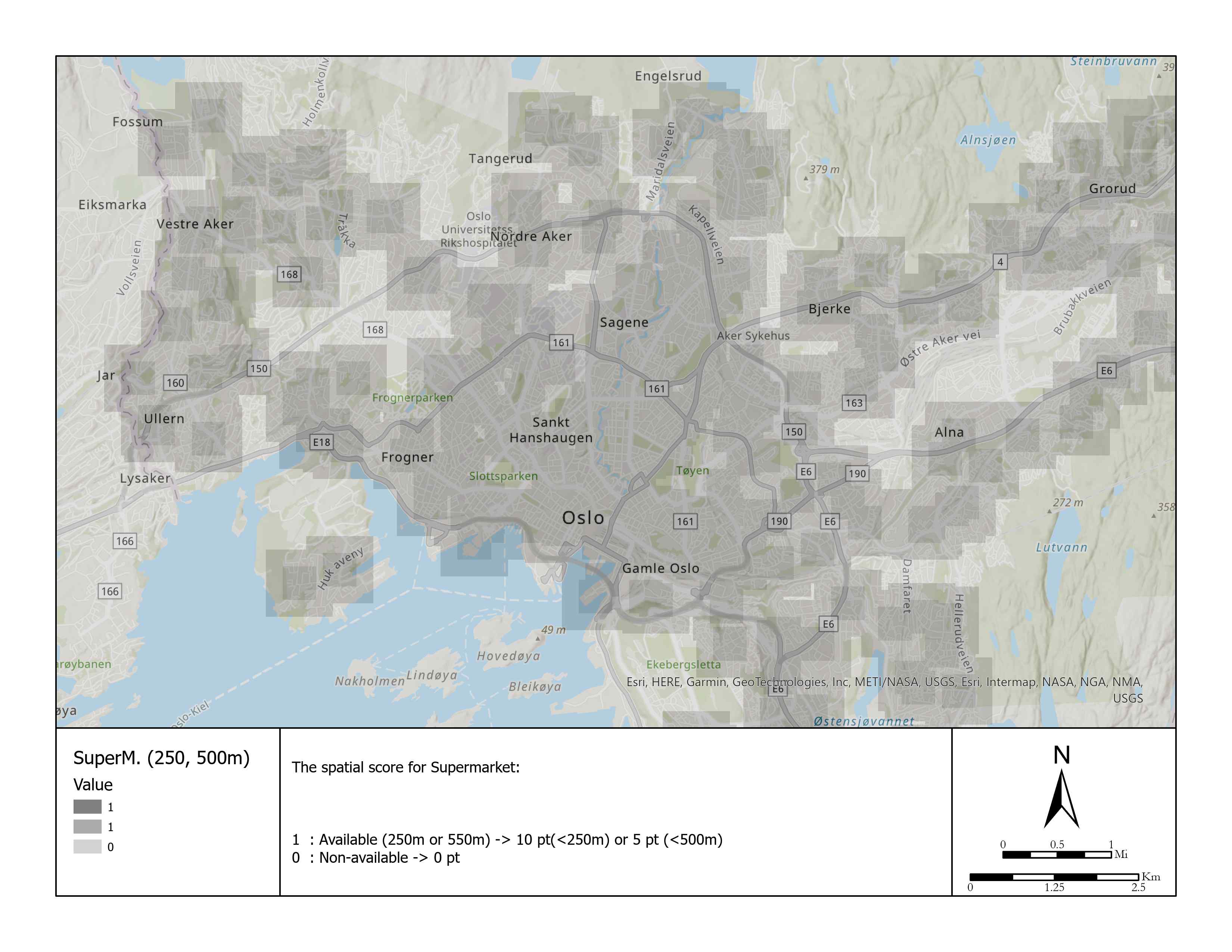
Shops and supermarkets.
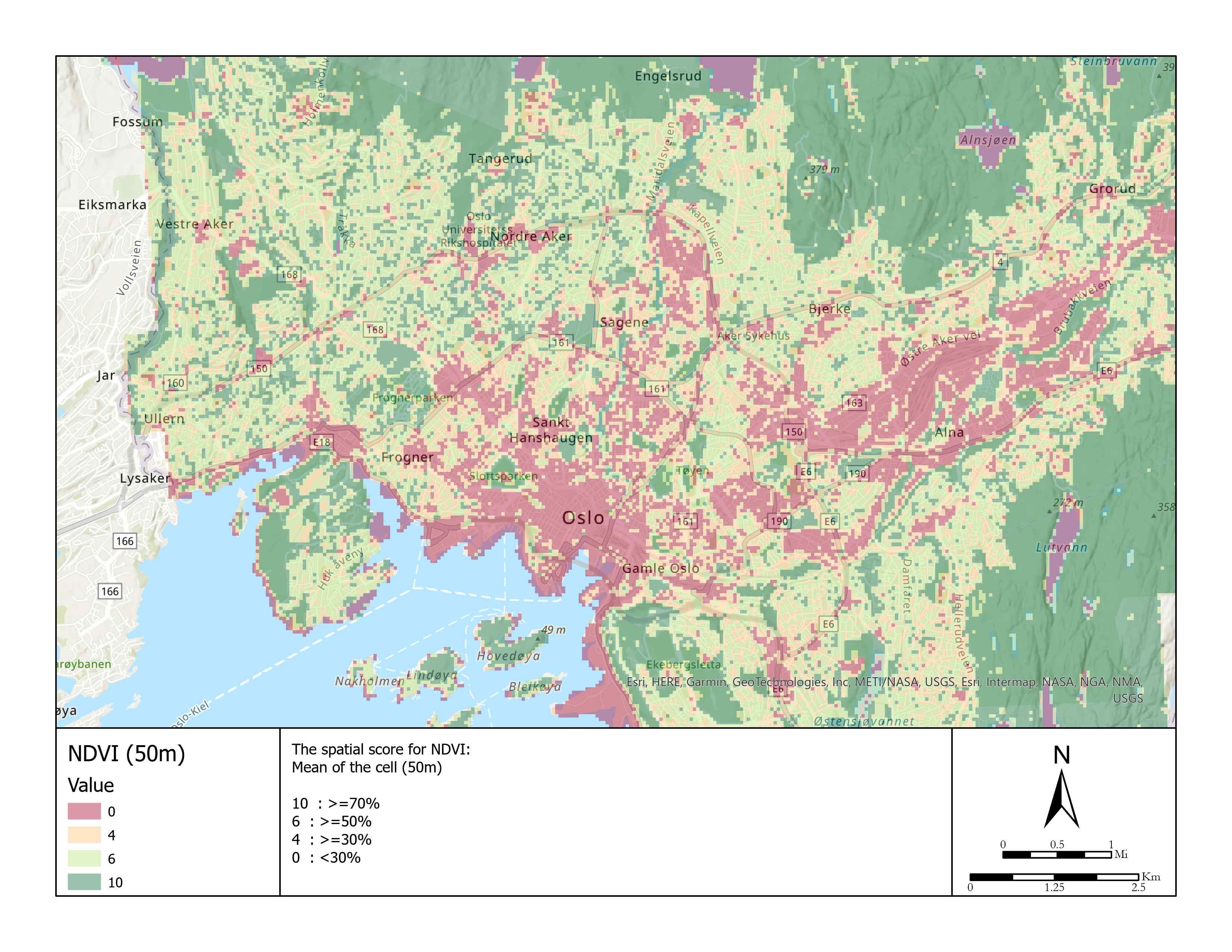
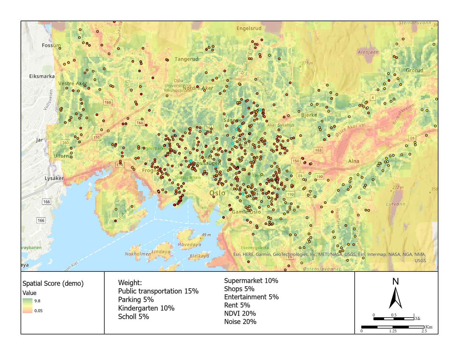
When we use NDVI as a criterion, there is an obvious underestimation for units located near the water body, e.g., shoreline or lake. For example, in Huk, the better view to fjord, the more expensive the house would be. However, the beach does not have any vegetation and does not contribute to the spatial score. This issue could be fixed by adding another criterion.
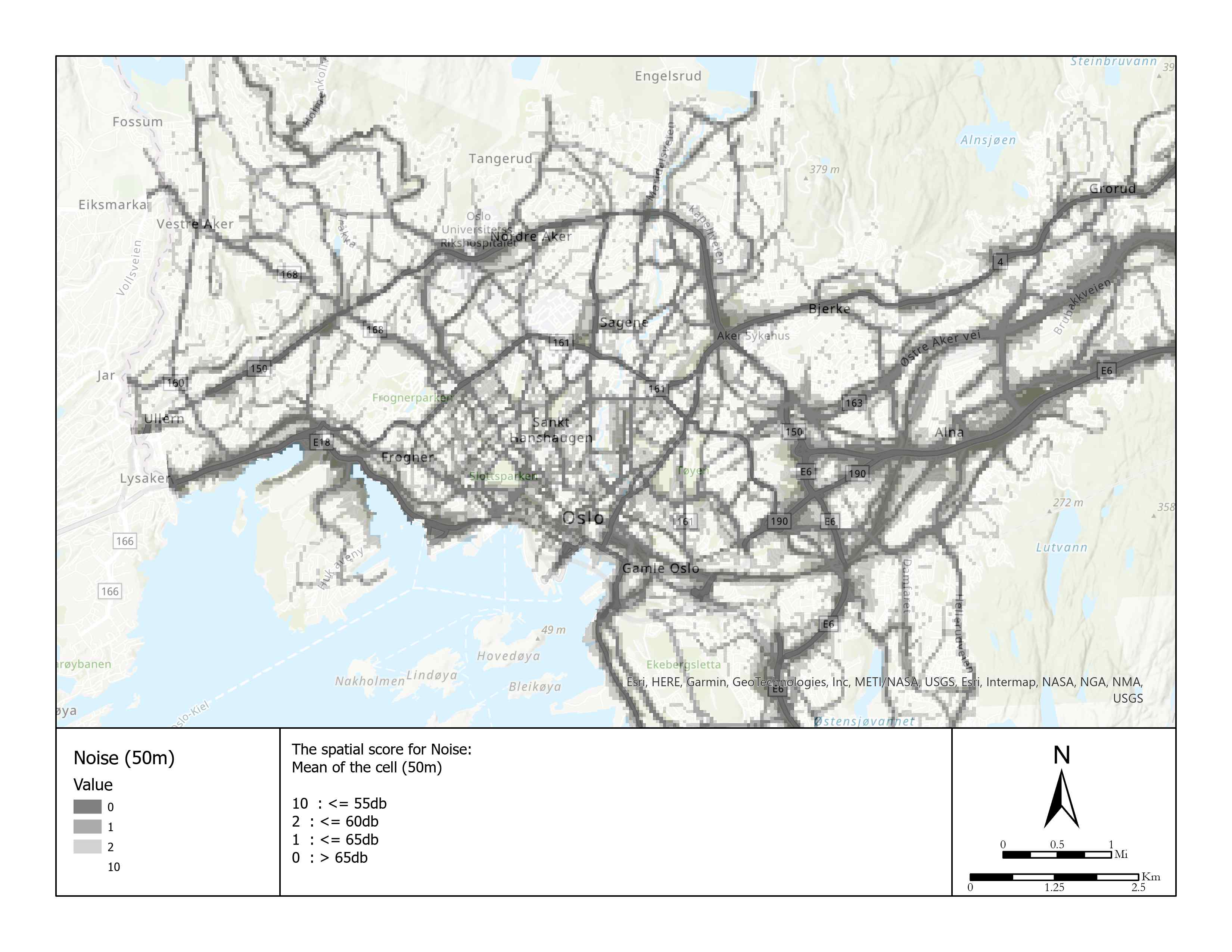
The average noise level below 55db over 24 hours would be thought harmless, 10 points, otherwise can only get 2 points (<60db), 1 point (<65db), 0 point (>65db). The noise exposure is the result from modeling, not indoor noise exposure, resulting in uncertainty about the final results. Since normally the noise model considers vegetation as an important parameter, the area close to parks and away from highways and railways get excellent scores from both two criteria.
What it suggests
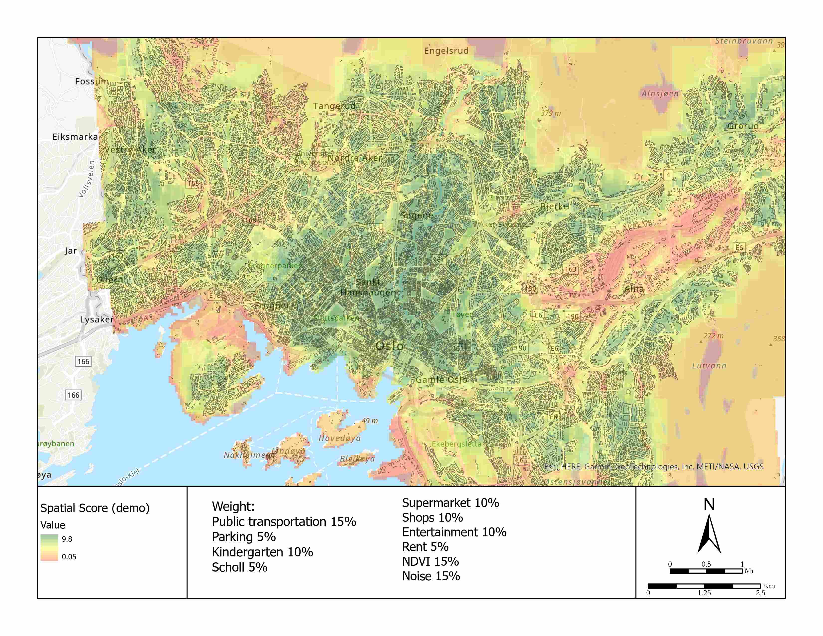
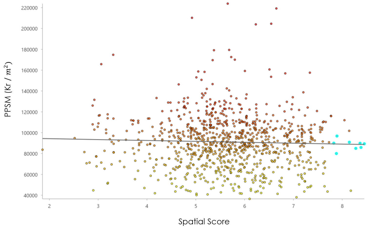
Aggregation was carried out under two scenarios, aggregation_1 based on demo parameters (table 1) and aggregation_2. When changing to the latter, shops, entertainment, NDVI and Noise were set from 5% to 10%, 5% to 10%, 20 % to 15% and 20% to 15%.
To be short, here is the recommended list of the units:
Table 2. The best-fits (Aggregation_1 > 8).
| Finn_code | District | Size | Price (Kr) | Type | Ppsm (Kr) | Aggregation_1 |
|---|---|---|---|---|---|---|
| 249110832 | Gamle Oslo | 71 | 6029516 | Andel • Leilighet • 3 soverom | 84923 | 8.28 |
| 248981927 | Frogner | 76 | 6909620 | Eier (Selveier) • Leilighet • 2 soverom | 90916 | 8.15 |
| 248049271 | Søndre Nordstrand | 81 | 3588916 | Eier (Selveier) • Leilighet • 2 soverom | 44308 | 8.18 |
| 249057789 | Sagene | 50 | 5088694 | Eier (Selveier) • Leilighet • 1 soverom | 101774 | 8.14 |
| 243905166 | Sagene | 53 | 4763626 | Andel • Leilighet • 1 soverom | 89880 | 8.36 |
| 248207270 | Sagene | 60 | 5362570 | Andel • Leilighet • 2 soverom | 89376 | 8.45 |
| 248035518 | Sagene | 95 | 8151292 | Eier (Selveier) • Leilighet • 3 soverom | 85803 | 8.38 |
There is a sensitivity test, using the second group of parameters:
Table 3. The best-fits (Aggregation_2 > 8).
| Finn_code | District | **Size ** | Price (Kr) | Type | Aggregation 2 | Aggregation 1 |
|---|---|---|---|---|---|---|
| 249110832 | Gamle Oslo | 71 | 6029516 | Andel • Leilighet • 3 soverom | 8.4 | 8.28 |
| 248219200 | Frogner | 84 | 9754142 | Eier (Selveier) • Leilighet • 2 soverom | 8.2 | 7.80 |
| 249057789 | Sagene | 50 | 5088694 | Eier (Selveier) • Leilighet • 1 soverom | 8.6 | 8.14 |
| 248999688 | Frogner | 36 | 3985861 | Andel • Leilighet • 1 soverom | 8.2 | 7.60 |
| 243905166 | Sagene | 53 | 4763626 | Andel • Leilighet • 1 soverom | 8.7 | 8.36 |
| 195629975 | - | 71 | 7483877 | Eier (Selveier) • Leilighet • 2 soverom | 8.1 | 7.50 |
| 248035518 | Sagene | 95 | 8151292 | Eier (Selveier) • Leilighet • 3 soverom | 8.6 | 8.38 |
Anything else?
A unit (finn code 248049271) at Søndre Nordstrand with extreme low price (3.6 million Kr) and good size (81 m2) got 8.18 points. Sadly, it is sold already. Most of the units recommend by model are sold already in the past month, which means the best-fit units are popular in some degree.
I know there are several issues in my method, but I have to limit my time on this project. Otherwise, a Web-based, automating GIS-MCDA model could be super fun for exploring dataset from Finn.
In general, the housing price MCDA model could provide the best-fitting options for house buyers but is not capable of suggesting selling price for landlords, because personnel preferences are totally different from the market average, and the model does not count the attributions of the house itself. But it is still possible and fun to do price estimation after gathering more information about market average and normalizing house attributions with coefficients.
